ONA in practice: turn a chapter-style figure into a reusable workflow.
The original ONA chapter, ENA tutorial article, and quantitative ethnography texts already explain the method in depth. This guide introduces those foundations more explicitly, then translates them into a stable, step-by-step workflow that researchers and AI agents can actually run: install, render, compare, troubleshoot, and reuse.
Guide author: Jewoong Moon (The University of Alabama, jmoon19@ua.edu)
ona R package's plot wrapper is broken on current Windows installs. We bypass it by calling its internal helpers directly — the math stays 100% authentic, only the rendering is rerouted.
An operational bridge to the canonical ONA literature.
The methodological heavy lifting already lives in the original sources: the ONA chapter, the ENA tutorial article, the quantitative ethnography book, and the package manuals for ona, tma, and rENA. This guide does not replace them. It reorganises them into an agent-friendly workflow with runnable templates, reproducible defaults, downloadable example files, and a practical workaround for the current Windows plotting failure. For theory and citation, defer to the originals in References.
The four views you can render
Every figure below was generated from the same reusable workflow pack and the same synthetic teacher–student dialogue dataset. Pick the view that matches your analytic question, then reuse the linked templates and starter files.


What is Ordered Network Analysis?
Ordered Network Analysis (ONA) is a quantitative ethnographic method developed by Tan, Swiecki, Ruis, and Shaffer (2024). It models how codes co-occur within a sliding temporal window — but unlike its predecessor, Epistemic Network Analysis (ENA), ONA preserves the direction of co-occurrence: which code preceded which.
That direction matters in any process where order is meaningful: classroom dialogue (who responded to whom), clinical decision-making (which symptom triggered which test), collaborative problem solving (whose contribution sparked which next move).
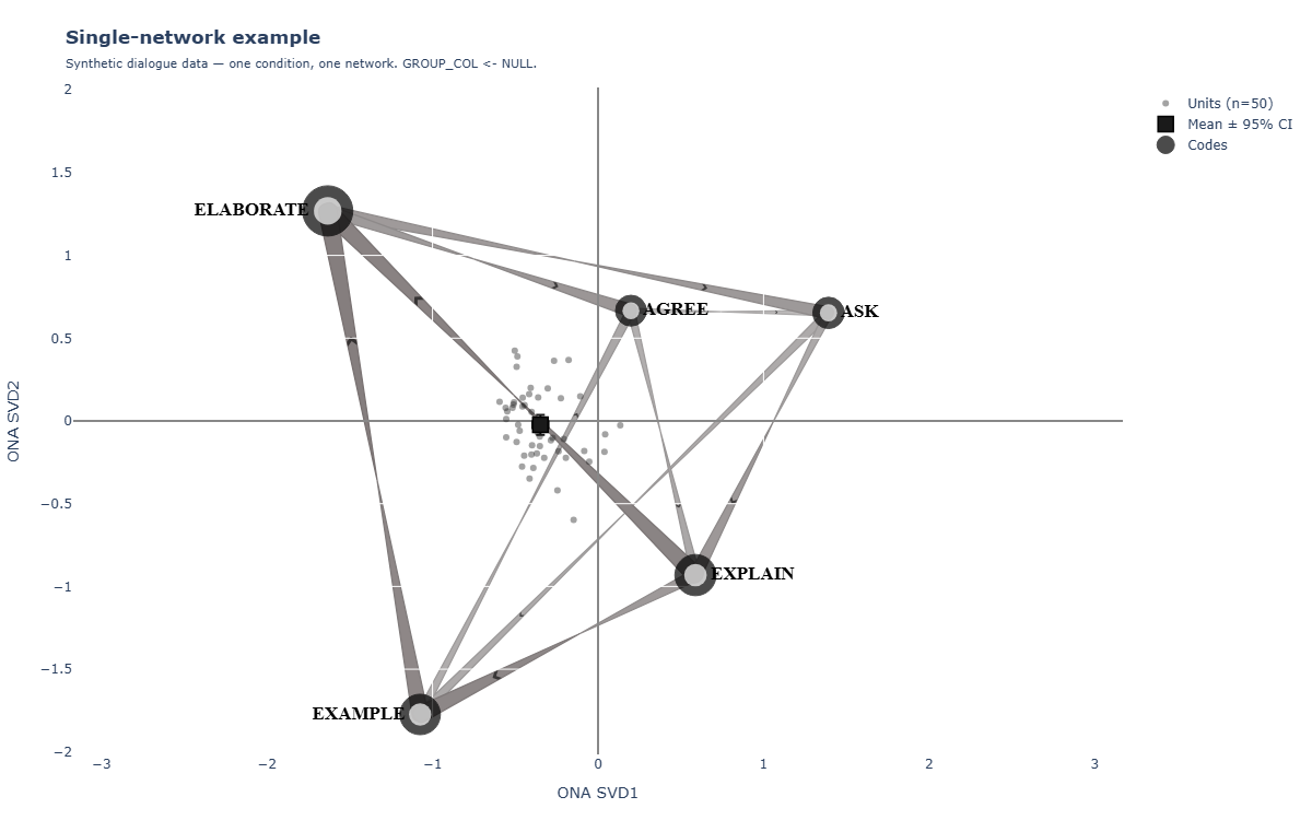
An ONA figure has four moving parts:
- Nodes are codes, positioned in a 2-D space derived from singular value decomposition (SVD) of the directional co-occurrence matrix. Codes that get co-occurrence pressure from similar partners cluster together.
- Edges are directional curved arrows that show "code X tended to follow code Y" — thicker arrow = stronger pull.
- Per-unit points are individual sessions/students projected into the same 2-D space — small dots scattered around the codes.
- Group means with 95% confidence intervals show where each condition's centroid sits in the projection.
The visual you see at the top of a typical ONA paper — directional curved arrows over a backbone of named codes, with two coloured groups overlaid or split into panels — is what this skill produces.
Why this guide, if the chapter and packages already exist?
The original ONA chapter and related ENA literature are strong on methodological explanation. They tell you what ONA is, why directional co-occurrence matters, and how to interpret the resulting network. What they do not try to be is a fault-tolerant, copyable workflow for contemporary R + Python environments or a prompt-ready workflow for AI agents.
That gap matters in practice. If you follow the official ona R-package plotting recipe on many current Windows machines, the build step succeeds but the wrapper silently produces an empty plot: the points appear, while arrows and node markers never inject into the layout.
I spent a long time trying to fix that wrapper directly — recompiling ona from source with RTools45, downgrading the package combo to the LAK24 versions, and swapping data.frame indexing for data.table indexing. None of it solved the operational failure.
Eventually I traced the failure into the wrapper's compiled logic: it builds the right edge geometry internally, then tries to inject it into a hierarchical legacy structure ($ENA_DIRECTION$response) that no longer matches the newer tma output. The injection silently fails, the figure renders empty, and no error is thrown.
The practical breakthrough: ona's internal helpers — create_edge_matrix(), edge_paths(), and to_square() — still work perfectly when called directly. They produce the same directional geometry and in-strength values the canonical figure depends on. This guide packages that working path into reusable templates, a one-shot driver, downloadable example files, and explicit instructions that an agent or a human collaborator can follow without guessing.
So the role of this guide is simple: keep the original literature as the conceptual authority, and make the workflow operationally reliable.
Do not call ona::nodes() or ona::edges() from this pipeline. They are silent no-ops on the current install and will give you an "empty figure" mystery that wastes hours.
Prerequisites & install
You need three things on your machine: R, Python, and (on Windows) RTools. The skill auto-detects the rest.
C:\Program Files\R\R-4.5.2\.C:\rtools45\. Needed once, in case any package needs to compile.install.packages(c("ona","tma","plotly","htmlwidgets","data.table","magrittr"))pip install -U plotly kaleido.Verify the install
From an R console:
# Should print version numbers (any 0.x is fine)
packageVersion("ona")
packageVersion("tma")
packageVersion("plotly")
From a terminal:
python -c "import kaleido; print(kaleido.__version__)"
# Expected: 1.x  — never 0.2.1
If print(kaleido.__version__) shows 0.2.1, the renderer will hang silently on Windows. Run pip install -U kaleido until it shows 1.x.
The skill includes a run_ona.ps1 driver that auto-detects your R install (4.4 / 4.5), checks kaleido, installs missing Python deps, then runs everything end-to-end. See Chapter 08.
Your data: the long-format CSV
ONA expects one row per turn (or whatever your atomic unit of "happening" is). Every code is a separate column with a 0/1 integer indicator. Plus identifying columns for unit, mode, and time.
Here is the minimal schema:
| Column | Type | What it carries |
|---|---|---|
| user_id | string / int | Who produced the turn. One value per session/participant. Used as the unit of analysis: each unique user_id becomes one ONA point. |
| cond | string | Group label. e.g. "AO" vs "non-AO", treatment vs control. Optional — drop if you only have one group. |
| turn_idx | integer | Monotonically increasing turn number within a session. Defines temporal order. The directional arrows depend on this. |
| speaker | string | Who is speaking on this turn. Used as the mode column so ONA can tell self-talk apart from cross-actor moves. |
| CODE_A | 0 / 1 | One column per code. 1 if the code applies to this turn, 0 otherwise. Repeat for every code (CODE_B, CODE_C, …). |
A worked example
Imagine a teacher–student dialogue with five codes (T_QUESTION, T_FEEDBACK, T_STATEMENT, S_QUESTION, S_RESPONSE). Your CSV starts like this:
user_id,cond,turn_idx,speaker,T_QUESTION,T_FEEDBACK,T_STATEMENT,S_QUESTION,S_RESPONSE
P01,AO,1,teacher,1,0,0,0,0
P01,AO,2,student,0,0,0,0,1
P01,AO,3,teacher,0,1,0,0,0
P01,AO,4,teacher,0,0,1,0,0
P02,non-AO,1,teacher,1,0,0,0,0
P02,non-AO,2,student,0,0,0,1,0
...
Keep all integer 0/1 code columns together at the right side of the CSV and metadata columns (id, group, time, speaker) at the left. The skill auto-discovers code columns by name, but a clean schema avoids future surprises.
The single-rule HOO concept
HOO stands for "head of output". It tells tma which past turns are eligible to send a directional connection to the current turn. In the chapter examples you'll see a two-rule pattern with separate ground and response rules. In our experience that pattern commonly errors out on real datasets when the ground/response conditions cannot both be satisfied for every turn.
The pattern that worked most reliably in the classroom, dialogue, and log-style datasets tested for this guide is one rule:
hoo <- tma:::rules(
  user_id %in% UNIT$user_id & cond %in% UNIT$cond
)
Read this as: "for every unit (a unique user_id × cond combination), the past turns eligible to send connections are exactly those that share the same user_id and the same cond." In plain words: connections only flow within a session, never across participants.
The skill template uses this pattern by default. Don't change it unless you know exactly why.
A worked dataframe you can run end-to-end
To make every figure in this guide reproducible, the skill ships a fully synthetic dialogue dataset at example_data/fake_dialogue_long.csv. It is not real data — transition matrices and group differences are designed by hand to produce a clean, interpretable ONA picture. Use it to verify your install before pointing the templates at your own data.
What it represents
A study with two conditions (treatment, control) and 50 participants per condition. Each participant produces 24–60 turns. Two speakers (A and B) take turns. Five codes describe what each turn does:
| Code | Meaning (illustrative) |
|---|---|
| ASK | The speaker asks a question of the partner. |
| EXPLAIN | The speaker offers an explanation or assertion. |
| EXAMPLE | The speaker provides a concrete example. |
| AGREE | The speaker agrees with the partner. |
| ELABORATE | The speaker extends, refines, or adds nuance. |
First ten rows
Read these rows like turns in a transcript. Each row is one turn. The five code columns are 0/1; exactly one is on per turn (in this synthetic data — in real data multiple codes can co-occur).
user_id, cond,      turn_idx, speaker, ASK, EXPLAIN, EXAMPLE, AGREE, ELABORATE
P001,    treatment, 1,        A,        1,   0,       0,       0,     0
P001,    treatment, 2,        B,        0,   1,       0,       0,     0
P001,    treatment, 3,        A,        0,   0,       1,       0,     0
P001,    treatment, 4,        B,        0,   0,       0,       0,     1
P001,    treatment, 5,        A,        0,   1,       0,       0,     0
P001,    treatment, 6,        B,        0,   0,       1,       0,     0
P001,    treatment, 7,        A,        0,   0,       0,       0,     1
P001,    treatment, 8,        B,        1,   0,       0,       0,     0
P001,    treatment, 9,        A,        0,   1,       0,       0,     0
P001,    treatment, 10,       B,        0,   0,       0,       1,     0
How to load it
# From R (matches the templates exactly)
long <- read.csv("path/to/fake_dialogue_long.csv",
                 stringsAsFactors = FALSE)
str(long)
# 'data.frame': 4136 obs. of 9 variables
Point any of the templates (ona_template.R, ona_panels_template.R, ona_subtracted_template.R) at this CSV with CODES = c("ASK","EXPLAIN","EXAMPLE","AGREE","ELABORATE") and GROUP_COL = "cond". The figures you get back should match the four views in the gallery at the top of this guide. If they don’t, your install is the problem — not your data.
ENA in five minutes — stanzas and the sliding window
ONA is a directional descendant of Epistemic Network Analysis (ENA). To read an ONA figure properly you need three ENA concepts: the stanza, accumulation, and projection. The R packages (tma behind the scenes) implement all three; you don’t set them by hand, but you do need to recognise them.
1. The stanza — what counts as "together"
A stanza is the local window of turns within which two codes are considered to co-occur. Two codes that fire 30 turns apart shouldn’t count as connected; two codes that fire in the same minute almost certainly should. The stanza is how ENA puts a number on "almost certainly."
The most common stanza definition is a sliding window of size w. For each turn, look at the previous w−1 turns. Every code that fired in that window is a "neighbour" of the current turn’s code(s). The skill’s templates use WINDOW_SIZE <- 4: each turn looks back three turns. Bigger window = more connections counted; smaller window = stricter "happened together." There is no universal best value — it depends on your turn granularity.
2. Accumulation — turning windows into a vector
Walk through every turn of every session, applying the stanza window. For each turn, increment the co-occurrence count for every (code-in-window, code-now) pair. After the walk, each unit of analysis (one session = one user_id×cond) has a vector of edge weights, one number per directed code pair.
For 5 codes there are 5×5 = 25 directed code pairs (including self-loops), so each session ends up as a 25-dimensional vector. With 100 sessions in the synthetic dataset, accumulation produces a 100-row, 25-column matrix.
3. Projection — SVD onto two axes
The 25-dimensional vectors are too many dimensions to look at. ENA applies singular value decomposition (SVD) to the matrix and keeps the two axes that explain the most variance — that’s SVD1 (x) and SVD2 (y) in every figure you see. Each session lands at a point in this 2-D space. The codes themselves are placed by a centroid rule: each node sits at the weighted average of the units that depend on it.
The result is what we’ve been looking at all along: codes as nodes in 2-D, sessions as small dots in the same 2-D, and edges weighted by the per-pair co-occurrence count.
Stanza → window → co-occurrence count → SVD → figure
You set the codes and the window. Everything else — accumulating co-occurrences, fitting SVD, placing nodes — happens inside tma when you call model(accum).
From ENA to ONA — what changes when you add direction
ENA treats co-occurrence as symmetric: if codes X and Y appear in the same window, the pair (X,Y) gets one count. ONA treats co-occurrence as directional: it matters whether X happened before Y or after.
That single change ripples through the whole pipeline.
| Step | ENA | ONA |
|---|---|---|
| Window | Symmetric: every code in the window pairs with every other code. | Asymmetric: only past–to–present pairs count. The "current" code is the receiver; everything in its lookback window is a sender. |
| Adjacency | k(k−1)/2 unordered pairs (off-diagonal). For 5 codes: 10 weights. | k² ordered pairs. For 5 codes: 25 weights (including self-loops). |
| Edge in the figure | Undirected line. Width = co-occurrence frequency. | Curved arrow with an arrowhead. Width = directional flow. |
| Node position | Centroid of the units that include the code. | Same SVD projection — positions are familiar to ENA users. |
| What the figure shows | "Which codes tend to appear together." | "Which codes tend to follow which." |
| Best for | Static co-occurrence patterns where order is meaningless. | Process data where order carries the meaning — dialogue, clinical workflow, gameplay sequences. |
Why direction matters — a concrete example
Imagine a tutoring session that contains both ASK and EXAMPLE. ENA can only tell you they appeared in the same stanzas often. ONA tells you something stronger:
- If the model says ASK → EXAMPLE is heavy, the tutor offers examples in response to learner questions — reactive scaffolding.
- If EXAMPLE → ASK is heavy instead, the tutor proactively shows examples, and questions follow — proactive scaffolding.
Both produce identical ENA figures. Only ONA distinguishes them.
Why the same projection works for both
ONA inherits ENA’s SVD-on-the-vector machinery: each session is still a long vector of edge weights, just twice as long because direction doubles the slots. The 2-D projection still lays codes out by centroid pull. So if you’ve read an ENA figure before, you already know how to read the layout. The only new visual element is the arrowhead.
Direction is computed inside tma whenever you pass mode.column = "speaker" and a numeric time.column. The same CSV that drives an ENA model can drive an ONA model — you just call model() on the directional accumulator. The skill’s templates already do this for you.
When to choose which
| Question you’re asking | Use |
|---|---|
| "Which constructs co-occur in this corpus?" | ENA |
| "Which moves trigger which other moves?" | ONA |
| "Did the treatment shift the order of operations?" | ONA |
| "Are these two corpora structurally similar?" | ENA (or ONA — both work) |
| "Who initiates and who responds?" | ONA + a speaker mode column |
| "What pairs often appear in the same window?" | ENA |
Everything in the rest of this guide is ONA-specific, but ENA users will recognise the bones.
An interactive ONA playground you can actually touch
This mini embed is not a full statistics engine. It is a reading tool for beginners: change the controls and watch how the same coded process looks different in combined, panels, and difference views.
Start in combined view, raise the threshold until only the dominant transitions survive, then switch to difference. If one code suddenly dominates the colored arrows, that is usually the structural story you should read first.
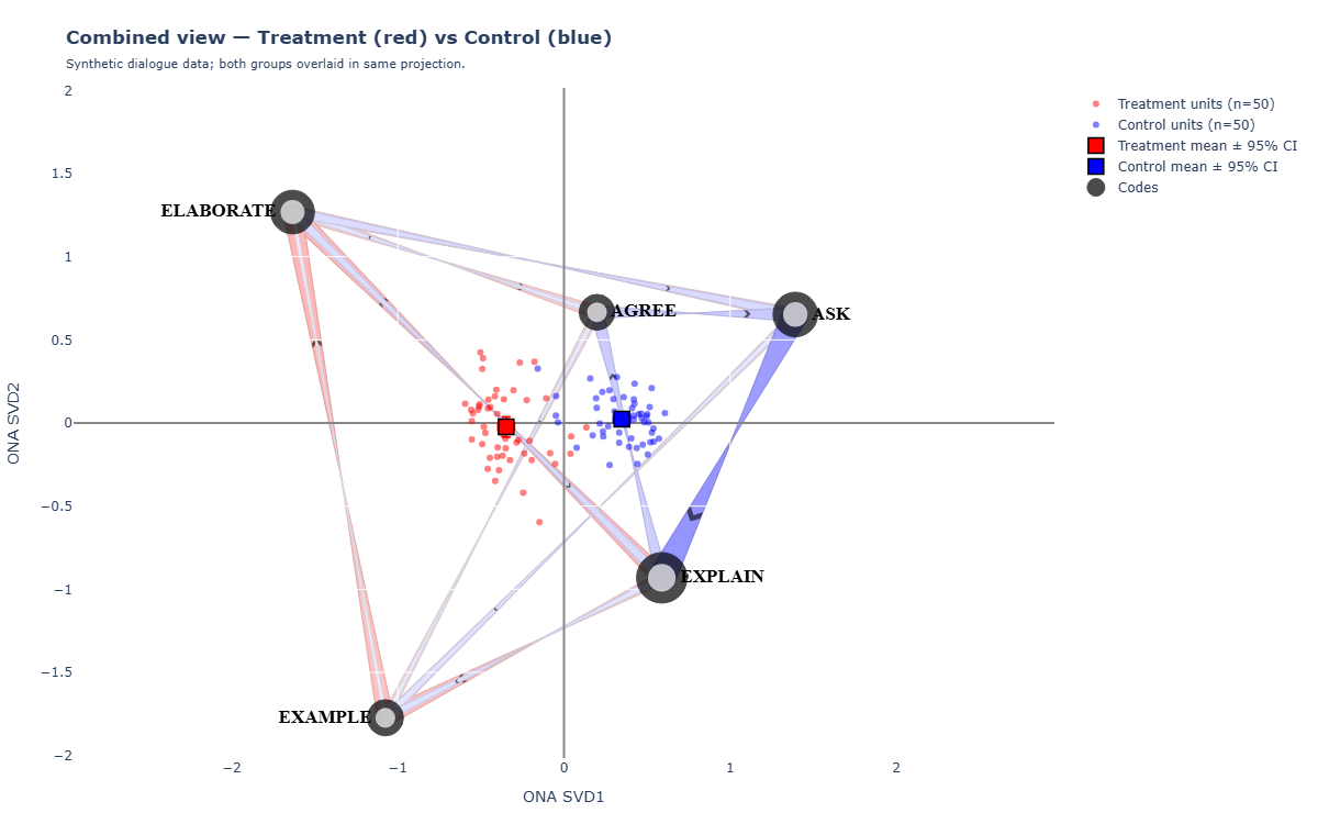
The combined view
This view overlays both groups' edges on the same plot — different colours, same node positions, same axis. Good when you want one figure that shows both group means in the same projection.
Step 1 · Copy the template
# From PowerShell, in your project root
Copy-Item "C:\Users\<you>\.claude\skills\ona\templates\ona_template.R" .\analysis\ona_run.R
Step 2 · Edit only the PARAMS block
Open analysis\ona_run.R in any editor and adjust the top section. Everything else can stay as-is on the first run.
# ---------------------------------------------------------------------------
# PARAMS — edit these
# ---------------------------------------------------------------------------
ROOT          <- "C:/Users/you/Desktop/MyProject"
CSV           <- file.path(ROOT, "data/turns_long.csv")
FIG_DIR       <- file.path(ROOT, "analysis/figures")
OUT_BASENAME  <- "ona_combined"

CODES         <- c("T_QUESTION","T_FEEDBACK","T_STATEMENT",
                 "S_QUESTION","S_RESPONSE")
UNIT_COLS     <- c("cond","user_id")
MODE_COL      <- "speaker"
TIME_COL      <- "turn_idx"
WINDOW_SIZE   <- 4

GROUP_COL     <- "cond"
G1            <- "AO"
G2            <- "non-AO"
EDGE_COLOR_1  <- "red"
EDGE_COLOR_2  <- "blue"
Step 3 · Run R
& "C:\Program Files\R\R-4.5.2\bin\Rscript.exe" .\analysis\ona_run.R
Expected console output:
Edge paths: 30 + 30
Node sizes: 25.8, 14.4, 26.2, 36.4, 46
Built figure: shapes = 60
[saved] ona_combined.html
[saved] ona_combined.json
Step 4 · Render the PNG
python "C:\Users\<you>\.claude\skills\ona\templates\render_ona_kaleido.py" ^
       .\analysis\figures\ona_combined.json ^
       .\analysis\figures\ona_combined.png 1200 750
You should now see ona_combined.png next to the JSON.
If your dataset has no group split, set GROUP_COL <- NULL and the template renders a single condition-agnostic mean network. The points and group-mean traces are skipped automatically.
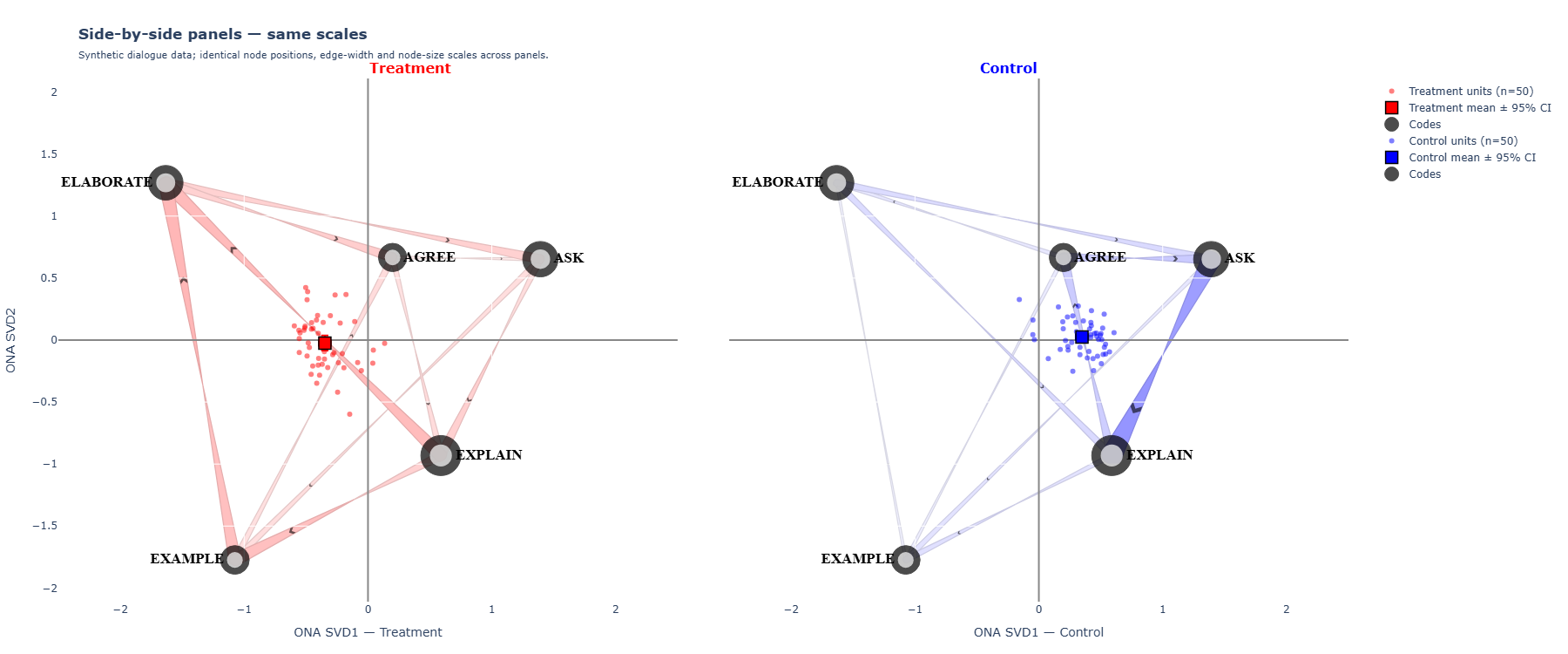
Side-by-side panels
When the combined overlay gets visually crowded — or when you need a fair group comparison for a figure caption — use the panels template. It draws two ONA networks side-by-side, with three things forced equal across panels:
Same node positions
Both panels use the same SVD rotation. A code that sits at the upper-left in panel 1 sits at the upper-left in panel 2.
Same edge-width scale
scale_edges_from = c(0, max(c(w_G1, w_G2))) — the thickest possible arrow in either panel maps to the same px width.
Same node-size scale
In-strength is summed across both groups (node_total = in1 + in2) so a node's diameter is comparable.
Edge colour + group mean
Panel 1 uses EDGE_COLOR_1, panel 2 uses EDGE_COLOR_2. Each panel shows only its own group's points and mean ± CI.
Run it
Copy-Item "C:\Users\<you>\.claude\skills\ona\templates\ona_panels_template.R" .\analysis\ona_panels_run.R
# edit PARAMS the same way as the combined template, then:
& "C:\Program Files\R\R-4.5.2\bin\Rscript.exe" .\analysis\ona_panels_run.R
python "C:\Users\<you>\.claude\skills\ona\templates\render_ona_kaleido.py" ^
       .\analysis\figures\ona_panels.json .\analysis\figures\ona_panels.png 1800 750
Note the wider canvas — 1800×750 instead of 1200×750 — to fit two panels.
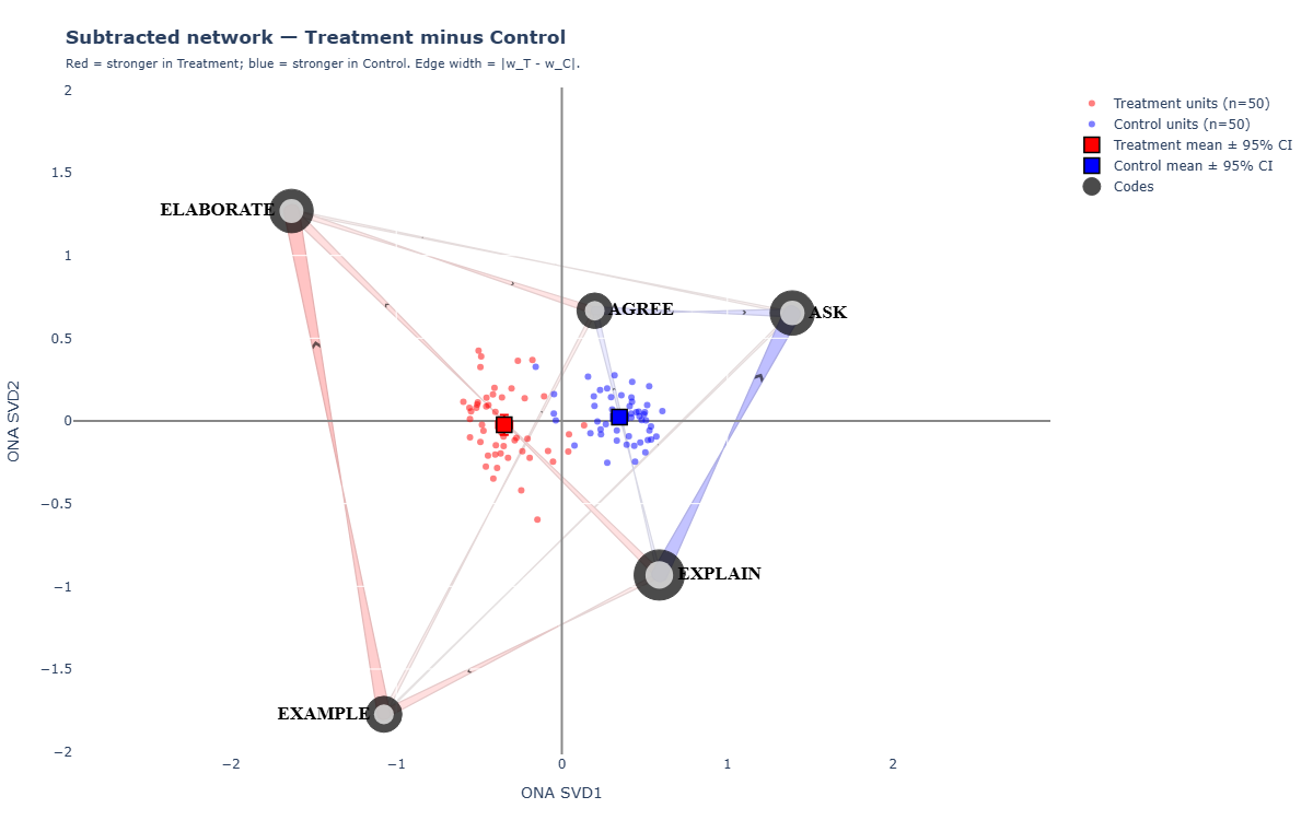
Subtracted (difference) network
The subtracted network is the canonical ONA group-comparison view. It encodes one number per edge: wG1 − wG2. Edges that are more frequent in G1 draw in EDGE_COLOR_1; edges that are more frequent in G2 draw in EDGE_COLOR_2. Edge width = absolute difference, so faint edges mean "the two groups behave nearly the same on this connection."
This is what you reach for when you want a single figure that answers: "how do the groups differ in dialogue structure?" The combined view shows both groups overlapping; the panels show each group cleanly; the subtracted view shows the shift.
Run it
Copy-Item "C:\Users\<you>\.claude\skills\ona\templates\ona_subtracted_template.R" .\analysis\ona_sub_run.R
# edit the same PARAMS as the other templates, then:
pwsh "C:\Users\<you>\.claude\skills\ona\templates\run_ona.ps1" ^
     -RScript .\analysis\ona_sub_run.R ^
     -OutDir .\analysis\figures ^
     -OutBaseName ona_subtracted
Expected console output (these are real numbers from a teacher-simulation dataset):
# Diff range tells you how big the per-edge differences are
Diff range: -0.2528 0.2407  | AO-favored: 12  | non-AO-favored: 13
Built subtracted network: shapes = 33
"AO-favored: 12 / non-AO-favored: 13"
Of the 25 directional edges in the model, 12 are stronger in the AO group and 13 are stronger in the non-AO group. The Diff range ±0.25 tells you the largest single-edge gap, which calibrates the colour saturation in the figure.
Some subtracted networks trigger a plotly.js error in kaleido due to near-zero edge geometries. The skill's render_ona_kaleido.py falls back to a Playwright screenshot of the saved HTML when this happens. The PNG you get is identical visually.
Per-function (per-actor) sub-networks
Once you have a working ONA model, you often want to ask narrower questions: "what happens if I look only at teacher-initiated moves?" or "what does the network look like for student responses only?" These are functional decompositions — slices of the same fitted model, redrawn with a subset of edges.
There are two ways to slice. Pick the one that fits your question.
"Show me edges where the SENDER is a teacher code"
Keep the same fitted model. Filter the directed adjacency matrix by row prefix (sender) or column prefix (receiver). Use the result as the weights vector for a fresh edge_paths call.
Best when your codes are already grouped by actor (e.g. T_*, S_*) and you just want to project a sub-graph.
"Refit ONA using only teacher-spoken turns"
Filter the long-format CSV upstream (long[long$speaker == "teacher", ]), then rerun the whole pipeline. You get fresh node positions, fresh SVD axes, fresh per-unit points.
Best when the actor's behaviour is qualitatively different and you want a separate model — but you lose comparability with the full network.
Option A · Code recipe (most common)
This snippet adds a "teacher-initiated only" sub-network to the standard pipeline. Drop it into your ona_run.R after the model is fit.
# Re-square the per-group weights into directed adjacency matrices
sq_ao <- ona:::to_square(ao_wts)   # rows = sender, cols = receiver
rownames(sq_ao) <- colnames(sq_ao) <- as.character(nodes_dt$code)

# Mask: keep only rows whose sender starts with "T_"
teacher_rows <- grepl("^T_", rownames(sq_ao))
sq_ao_T <- sq_ao
sq_ao_T[!teacher_rows, ] <- 0   # zero out non-teacher senders

# Convert back to a flat weight vector in the same order ona expects
ao_wts_T <- as.numeric(t(sq_ao_T))     # row-major flatten

# Build edge paths for this sub-network
em_T <- ona:::create_edge_matrix(NULL, weights = ao_wts_T,
                                  nodes = nodes_dt, direction = 1)
ep_T <- ona:::edge_paths(em_T, edge_color = c("darkgreen"),
   edge_size_multiplier = 0.4, scale_edges_to = c(0,1.5),
   scale_edges_from = c(0, max(ao_wts_T)), # ... rest of params same)
Then add ep_T to your shapes_combined list. The result: a figure where only teacher-initiated arrows are visible, painted in green, against the same node positions as the main figure.
Common functional cuts to consider
| Question | Slice | Mask used |
|---|---|---|
| Teacher-initiated moves only | Sender = T_* | grepl("^T_", rownames(sq)) |
| Student-initiated moves only | Sender = S_* | grepl("^S_", rownames(sq)) |
| Cross-actor moves | T→S or S→T | Mask out same-prefix sender↔receiver pairs |
| Reciprocal exchanges | X→Y AND Y→X both present | (sq > 0) & (t(sq) > 0) |
| Sink-only edges | Receiver = highest in-strength code | Keep only the column matching the top-in-strength code |
| Self-loops | Sender = Receiver | diag(sq) |
When you slice (Option A), keep the node positions, axis range, and per-unit points from the full fitted model. That way the sub-network is interpretable in the same projection — readers can compare a teacher-only figure against the all-actors figure code-for-code.
The one-shot driver
If you don't want to remember the Rscript path or the kaleido install line every time, use run_ona.ps1. It auto-detects an R 4.4+ install, ensures Python deps, runs your R script, then renders the PNG.
pwsh "C:\Users\<you>\.claude\skills\ona\templates\run_ona.ps1" ^
     -RScript ".\analysis\ona_run.R" ^
     -OutDir ".\analysis\figures" ^
     -OutBaseName "ona_combined" ^
     -Width 1200 -Height 750
One line. The driver prints what it does:
[ona] Rscript: C:\Program Files\R\R-4.5.2\bin\Rscript.exe
[ona] running R: .\analysis\ona_run.R
Edge paths: 30 + 30
Node sizes: 25.8, 14.4, 26.2, 36.4, 46
Built figure: shapes = 60
[ona] rendering PNG via kaleido ...
[saved] .\analysis\figures\ona_combined.png
[ona] DONE: .\analysis\figures\ona_combined.png
For panels just point -RScript at the panels run-file and bump -Width to 1800.
The tuning knobs you can change
The defaults are chosen to match the chapter Fig 4 aesthetic. If you want something different, here is what each knob does and what range stays sensible.
| Knob | Default | What it controls |
|---|---|---|
| EDGE_SIZE_MULT | 0.4 | Multiplier inside edge_paths. Bigger → fatter arrows overall. Range 0.2–0.8. |
| EDGE_SCALE_TO | c(0, 1.5) | Output range for edge widths. Bumping the upper bound makes the strongest edge thicker without touching the weakest. |
| EDGE_LINE_MULT | 2.5 | Extra multiplier applied to line.width when shapes are emitted to plotly. Useful if you want bolder strokes without changing the underlying edge geometry. |
| NODE_SIZE_MIN | 12 | Smallest possible node diameter (in px). The least-connected node draws at this size. |
| NODE_SIZE_RANGE | 34 | Span above the minimum. Maximum node = MIN + RANGE = 46 px by default. |
| DONUT_INNER_RATIO | 0.55 | Inner white circle relative to outer. Smaller → thicker ring. |
| LABEL_FONT_PX | 17 | Code-label font size in px (serif). Bump for poster-size figures. |
All seven of these live in the PARAMS block at the top of each template. You don't have to touch the rest of the script.
Pitfalls & how to recover
Any of these can happen on a fresh setup. Each one has a fast diagnostic and a one-line fix.
The PNG is empty (axes only, no arrows, no nodes)
Cause: You called ona::nodes() / ona::edges() somewhere. Those wrappers silent-fail.
Fix: Rerun using one of the skill templates as your starting point. The templates never call those wrappers.
module 'kaleido' has no attribute 'scopes'
Cause: kaleido 0.2.1 is installed.
Fix: pip install -U kaleido until the version reports as 1.x.
R errors: ENA_DIRECTION not found
Cause: You data.frame-indexed set$line.weights with [df$col == "X", ]. That syntax strips the ena.line.weights class.
Fix: Use the template's pattern — extract the numeric matrix via as.matrix() and aggregate with colMeans().
All edges are zero / no arrows render
Cause: The HOO rule excluded every turn (no co-occurrences passed the filter).
Fix: In R, print nrow(flat) and range(ao_wts). If the matrix is empty, your UNIT_COLS or cond filter is too strict — relax it.
Nodes hide behind the edges
Cause: layer = "below" got dropped from the shape spec, or marker sizemode defaulted to "area" and shrunk the donut hole.
Fix: Restore both lines from the template; do not edit them.
Rscript: command not found
Cause: Rscript is not on PATH on Windows by default.
Fix: Use the absolute path "C:\Program Files\R\R-4.5.2\bin\Rscript.exe", or use run_ona.ps1 which auto-detects.
Network metrics — what numbers can you pull out?
The figure is one expression of the model. The same model carries node-level and network-level summary statistics you can drop into a Results table or a regression model. The skill ships templates/ona_metrics.R which produces all of them.
Node-level metrics — per code, per group
For each code, you get four numbers per group plus two differences:
| Metric | R | What it tells you |
|---|---|---|
| in-strength | colSums(sq) | How much directional weight the code receives. The "sink" of the field. |
| out-strength | rowSums(sq) | How much directional weight the code initiates. The "source" of the field. |
| total degree | in + out | Combined participation. Drives the donut node size in the figure. |
| in_diff | in_G1 − in_G2 | Where the receiving load shifted across groups. |
| out_diff | out_G1 − out_G2 | Where the sending load shifted across groups. |
Real example from a teacher–student dialogue dataset (AO = treatment, non-AO = control):
          in_T   out_T  in_C   out_C  in_diff  out_diff
ASK       0.597  0.633  1.147  1.174  −0.549  −0.541
EXPLAIN   0.919  0.917  1.154  1.133  −0.235  −0.216
EXAMPLE   0.896  0.879  0.381  0.359  +0.515  +0.520
AGREE     0.580  0.587  0.672  0.674  −0.092  −0.088
ELABORATE 1.216  1.192  0.476  0.488  +0.740  +0.704
How to read this table in plain words:
- ELABORATE is the biggest treatment-favoured sink (in +0.74). Treatment dialogues route a lot more flow into elaboration moves.
- EXAMPLE jumps the same direction (+0.52 in / +0.52 out). Together with ELABORATE this is a structural fingerprint of the treatment: explain → give an example → elaborate.
- ASK moves the opposite way (−0.55 in / −0.54 out). Control dialogues lean more on question-asking; treatment displaces that load onto example-and-elaborate sequences.
Network-level metrics — per group
| Metric | What it captures |
|---|---|
| Active edges | Count of edges with weight > 0. Maximum is k² for k codes (here 25 for 5 codes). |
| Total mass | sum(weights) — the cumulative co-occurrence pressure in the network. Compare relative mass across groups; absolute values depend on units. |
| Density | Fraction of possible edges with non-zero weight. Density = 1 means every code reaches every other code at some point. |
| Mean SVD1 / SVD2 | Where the group's centroid sits in the projection. Drives the square-marker means in the figure. |
| Between-means distance | Euclidean distance between the two group means. The headline "how far apart are these groups?" number. |
From the same dataset:
             metric    Treatment    Control
       Active edges       25           25
         Total mass        4.21         3.83
            Density        1.00         1.00
          Mean SVD1       −0.348       +0.348
          Mean SVD2       −0.024       +0.024
 Between-means dist        0.698        —
Both networks are equally dense and carry similar total mass — the difference is where the mass goes, not how much. That's a typical ONA finding: the structure shifts even though the volume stays comparable.
The per-unit SVD1/SVD2 coordinates and the per-unit in/out-strength of any code are valid outcome variables for a downstream regression — e.g. predict SVD1 position from condition + covariates. ONA gives you the structure; the regression gives you the inference.
Group comparison statistics
The figure shows where two groups land in the projection. The numbers below tell you whether that separation is reliable. Three tests are standard. The skill's ona_metrics.R runs all three.
Welch's t-test on SVD1 / SVD2
Tests whether the per-unit mean coordinate differs between groups, allowing unequal variances. Reasonable default when units are roughly normally distributed in each group.
t.test(SVD1 ~ cond, data = pts_df)
t.test(SVD2 ~ cond, data = pts_df)
Mann–Whitney U
Drop the normality assumption — tests whether one group's coordinates tend to be higher than the other. Use this when n is small or when residuals are skewed.
wilcox.test(SVD1 ~ cond, data = pts_df)
wilcox.test(SVD2 ~ cond, data = pts_df)
Cohen's d
p-values shrink with sample size. Cohen's d gives you the magnitude of the difference in pooled-SD units. Conventional anchors: 0.2 small, 0.5 medium, 0.8 large.
# pooled-SD effect size
(mean(x) - mean(y)) /
  sqrt(((nx-1)*var(x) + (ny-1)*var(y))
       / (nx+ny-2))
Randomization test on the between-means distance
The most defensible test for ONA: repeatedly shuffle the condition labels, recompute the between-means distance, and ask "how often does chance produce a separation as large as the one we observed?"
obs_d <- sqrt(sum((m1 - m2)^2))
perm_d <- replicate(2000, {
  s <- sample(pts_df$cond)
  ...
})
p <- mean(perm_d >= obs_d)
Real output (B = 2000 permutations)
# GROUP COMPARISON STATISTICS (synthetic data)
 axis    t_stat    t_p     cohen_d
 SVD1   +20.076  <.0001   −4.015
 SVD2    +1.333   .1863   −0.267

# PERMUTATION TEST (B = 2000)
  Observed dist:   0.698
  Null mean (95%): 0.074 (0.012, 0.182)
  p-value:         < .0001

# Sign convention: R t.test(y ~ cond) compares first level (control)
# minus second level (treatment); with control mean > treatment mean on SVD1,
# t is positive. Cohen's d here is treatment − control, so it is negative.
Read like this:
- SVD1 separation is enormous (Cohen's d ≈ 4.0, far past the conventional "large effect" threshold of 0.8). With cleanly differentiated synthetic transition matrices, the test correctly detects them.
- SVD2 separation is essentially null (d ≈ 0.27, p ≈ .19). The synthetic groups overlap on the secondary axis — a useful sanity check that the test isn’t trigger-happy.
- The overall separation is far beyond chance: observed between-means distance 0.70 vs permutation null mean 0.07 (95th percentile 0.18).
SVD1 is the axis that maximally separates the network on first read. If you change the rotation (e.g. mean-rotated vs SVD-rotated, or a custom rotation node), the t-test answer changes too. Report which rotation you used — and don't compare t-statistics across different rotations.
Interpretation framework
An ONA figure looks like a network diagram, but the right way to read it is as a structural fingerprint of how codes flow into each other. Use this five-pass framework. Each pass answers one question; do them in order.
A worked interpretation
Using the same teacher-simulation data shown above, here is how a Results paragraph might read after walking the framework:
"The ONA mean networks show that the Treatment and Control sessions occupy structurally different regions of the projection (between-means distance = 0.70, permutation p < .001). The separation is concentrated on the first SVD axis (Cohen’s d = −4.02) rather than the second (d = −0.27). Inspecting node-level in-strength differences, the contrast is driven by ELABORATE (+0.74), EXAMPLE (+0.52), and ASK (−0.55): under the treatment, dialogues route flow into example→elaborate sequences while question-asking declines. The subtracted network confirms that EXPLAIN → EXAMPLE and EXAMPLE → ELABORATE arrows are systematically thicker in the Treatment group, while ASK-initiated arrows dominate the Control group. We interpret this as a shift in dialogue structure — not as evidence of a causal effect on outcomes, which would require the study design to support it. (Numbers above are from the synthetic dataset bundled with the skill; replace with your own.)"
When to be cautious
| Symptom | Risk | What to do |
|---|---|---|
| One group has < 15 units | Means are unstable | Bootstrap the means or report rank-based tests only. |
| The two means' CIs overlap heavily | The visual separation may be illusory | Lead with the permutation p, not the eyeballed gap. |
| SVD1 separation is large but SVD2 is null | Real, but interpret only on the axis that separates | Don't claim the groups differ "everywhere" — they differ on one axis. |
| One group dominates total mass | The other group has more zero-weight edges, density looks artificially low | Report active-edge counts side-by-side; consider matching session lengths. |
| Codes are extremely sparse (mostly 0) | The window-based co-occurrence is noisy | Increase the window size or merge low-frequency codes upstream. |
| Groups differ on something the design didn't randomize | Whatever you observe might be confounded | Stay descriptive in the abstract. Causal claims require a causal design. |
ONA is a descriptive method. A well-separated network tells you the groups look structurally different. It does not tell you why, and it does not license a causal claim unless your design supports one independently.
Cheat sheet
install.packages(c(
  "ona","tma","plotly",
  "htmlwidgets","data.table"
))
# in a terminal
pip install -U plotly kaleido
pwsh run_ona.ps1 ^
  -RScript .\ona_run.R ^
  -OutDir .\figures ^
  -OutBaseName ona_combined
& "C:\Program Files\R\R-4.5.2\bin\Rscript.exe" ona_run.R
python render_ona_kaleido.py ^
       figures\ona_combined.json ^
       figures\ona_combined.png 1200 750
user_id, # unit identity
cond,    # group (optional)
turn_idx,# numeric time
speaker, # mode
CODE_A, CODE_B, ...   # 0/1 ints
Where each file lives
| SKILL.md | The skill's dispatch doc — read by Claude / Codex when triggered. |
| templates/ona_template.R | Combined-view R script. Copy + edit PARAMS. |
| templates/ona_panels_template.R | Side-by-side panels with shared edge/size/position scales. |
| templates/ona_subtracted_template.R | Group-difference (subtracted) network. Red = G1-favored, blue = G2-favored. |
| templates/ona_metrics.R | Node + network metrics + group comparison statistics + permutation test → CSVs. |
| templates/render_ona_kaleido.py | kaleido 1.x PNG renderer. No edits needed. |
| templates/run_ona.ps1 | One-shot driver: env detect + R + render. No edits needed. |
| GUIDE.html | This document. |
If everything ran cleanly, you now have a publication-quality ONA figure. Open the HTML version too — it's interactive in a browser.
References — cite the originals
This guide stands on the work of the Epistemic Analytics group at the University of Wisconsin–Madison and contributors to the open-source ona, tma, and rENA R packages. If you publish work that uses these tools, please cite the canonical sources below — not this guide.
Methodological foundations
- ONA — Ordered Network Analysis. Tan, Y., Swiecki, Z., Ruis, A. R., & Shaffer, D. W. (2024). Ordered network analysis. In B. Wasson & S. Zörgő (Eds.), Advances in quantitative ethnography. (Chapter / book series.) Introduces ONA as a directional extension of ENA; the figure conventions reproduced here come from this chapter. Verify exact bibliographic details against the published volume before citing.
- ENA — Epistemic Network Analysis. Shaffer, D. W., Collier, W., & Ruis, A. R. (2016). A tutorial on epistemic network analysis: Analyzing the structure of connections in cognitive, social, and interaction data. Journal of Learning Analytics, 3(3), 9–45. https://doi.org/10.18608/jla.2016.33.3
- Quantitative ethnography (book). Shaffer, D. W. (2017). Quantitative ethnography. Cathcart Press. The methodological framing under which ENA and ONA sit.
- Transmodal analysis (TMA). The accumulation pipeline behind
tmageneralises ENA to multimodal and directional data. Please consult the package author list, accompanying papers, and the CITATION file when citing the method.
Software
onaR package. Tan, Y., Marquart, C. L., Ruis, A. R., Cai, Z., Knowles, M. A., Eagan, B., & Shaffer, D. W. ona: Ordered Network Analysis. CRAN. cran.r-project.org/package=ona — in R, runcitation("ona")to get the version-specific citation block.tmaR package. tma: Transmodal Analysis. CRAN. cran.r-project.org/package=tma —citation("tma").rENAR package. Marquart, C. L., Swiecki, Z., Collier, W., Eagan, B., Woodward, R., & Shaffer, D. W. rENA: Epistemic Network Analysis. CRAN. cran.r-project.org/package=rENA —citation("rENA").- Epistemic Network Analysis (web tool). epistemicnetwork.org — the maintained web application from the Epistemic Analytics group.
- Plotly & Kaleido. Used here purely for figure rendering. plotly.com · github.com/plotly/Kaleido.
Implementation notes this guide leans on
- The LAK24 teacher-practices repository by A. Hussain (Wisc.) is a useful real-world example of
ona/tmausage and inspired the data.table-based subsetting pattern reused here. - The figure aesthetic borrows the knowledge-arch-blueprint theme tokens from nexu-io/open-design (MIT licensed) — cream paper background, rust-red highlights, blueprint grid.
Why this guide helps in agentic workflows
The chapter, articles, and package docs above are the right places to learn the method. This guide exists because agentic execution needs a different layer of support: explicit file contracts, fixed parameter blocks, reproducible defaults, predictable output names, and troubleshooting rules that prevent silent failure. In other words, the canon explains what ONA means; this guide explains how to get a trustworthy ONA artifact out of a real machine and hand it off to an AI workflow without ambiguity.
Downloadable starter files
Full sanitized workflow bundle
Download the ONA agentic starter pack (.zip) — includes the sanitized skill example, core templates, renderer, driver, synthetic dataset, generator script, and example output PNGs.
No personal information
Download a public-safe ONA skill example (.md) that shows the trigger rules, workflow logic, and operational defaults without any personal notes or private project content.
Synthetic long-format CSV
Download the synthetic ONA dialogue dataset (.csv) or download the generator script (.py) if you want to inspect or regenerate the example data.
Directly reusable files
Combined template (.R), panels template (.R), one-shot driver (.ps1), and kaleido renderer (.py).
Preview the outputs first
Single network (.png), combined network (.png), panel comparison (.png), and subtracted network (.png).
Render all examples
Download the batch render script (.R) if you want one file that reproduces the example outputs against the bundled synthetic data.
How to cite this guide (optional)
If you must cite this on-ramp itself (e.g., for a tutorial or class handout), use:
Educatian. (2026). ONA in Practice — reproducible ONA workflows for researchers and agents
   [Open guide]. https://educatian.github.io/ona/
But for any methodological claim, defer to the original sources above.
This is a community on-ramp, not the canonical source.
Numbers in this guide come from a synthetic dataset bundled here for demonstration. Wording is summarised in our own words to be beginner-accessible. Anything you find in conflict with the original publications or the package manuals: trust the originals, and please open an issue / send a correction.